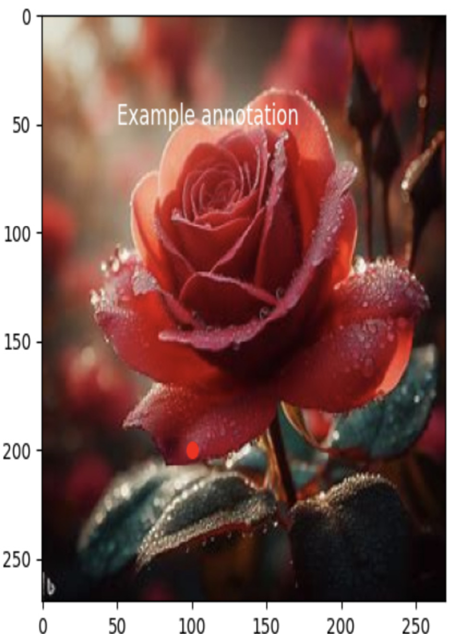
We can add annotations to an image to highlight specific regions of interest, such as marking key features within an image, perhaps facial landmarks on a person’s face (eyes, nose, mouth), to emphasize important attributes for analysis or recognition. Annotations can also be used to highlight regions that exhibit anomalies, defects, or irregularities in industrial inspection images, medical images, and quality control processes, along with identifying and marking specific points of interest, such as landmarks on a map. Let’s see annotations at work:
import matplotlib.pyplot as plt
import numpy as np
from PIL import Image
# Load an image
img = Image.open(‘../images/roseflower.jpeg’)
# Convert image to numpy array
img_array = np.array(img)
# Plot the image with annotations
plt.imshow(img_array)
plt.scatter(100, 200, c=’r’, s=50)
plt.annotate(“Example annotation”, (50, 50), fontsize=12, color=’w’)
plt.show()
We get the following result as output:

Figure 4.6 – Image annotation
These are just a few examples of the many ways that we can use Matplotlib to visualize image data. With some creativity and experimentation, we can create a wide variety of visualizations to help us understand our image data better.
Practice example of image segmentation
The following simple code snippet demonstrates how to perform basic image segmentation using the CIFAR-10 dataset and a simple thresholding technique:
import numpy as np
import matplotlib.pyplot as plt
from keras.datasets import cifar10
# Load the CIFAR-10 dataset
(x_train, _), (_, _) = cifar10.load_data()
# Select a sample image for segmentation
sample_image = x_train[0] # You can choose any index here
# Convert the image to grayscale (optional)
gray_image = np.mean(sample_image, axis=2)
# Apply a simple thresholding for segmentation
threshold = 100
segmented_image = np.where(\
gray_image > threshold, 255, 0).astype(np.uint8)
# Plot the original and segmented images
plt.figure(figsize=(8, 4))
plt.subplot(1, 2, 1)
plt.imshow(sample_image)
plt.title(‘Original Image’)
plt.subplot(1, 2, 2)
plt.imshow(segmented_image, cmap=’gray’)
plt.title(‘Segmented Image’)
plt.tight_layout()
plt.show()
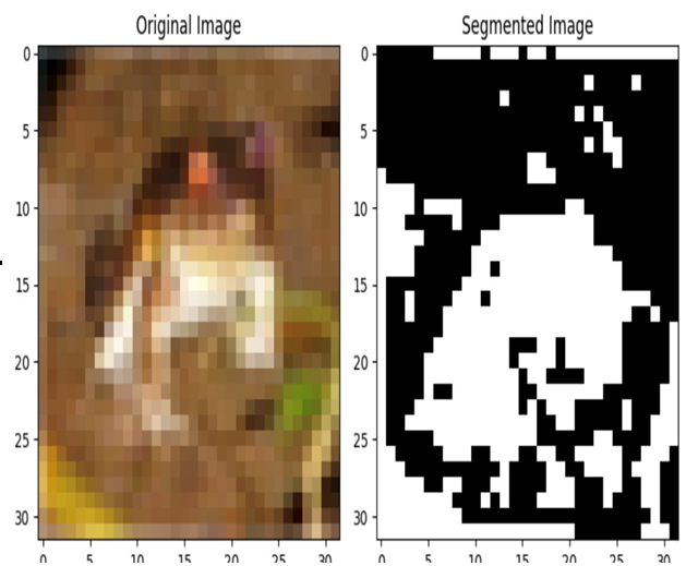
The result is as follows:

Figure 4.7 – Image segmentation
This example uses a basic thresholding technique to segment the image based on pixel intensity values.
